

ApiNATOMY User Guide
Physiology deals with the body in terms of anatomical compartments that delineate portions of interest. The compartments can be defined at various anatomical scales, from organs to cells. Clinical and bioengineering experts are interested to see records of physical measurements associated with certain anatomical compartments.
ApiNATOMY is a methodology to coherently manage knowledge about the scale, parthood and connectivity of anatomical compartments as well as to represent and analyse process mechanisms and associated measurements. It consists of
- a knowledge model about biophysical entities, and
- a method to build knowledge representations of physiology processes in terms of biophysical entities and physical operations over these entities.
The following Youtube video explains the ideas underlying the ApiNATOMY methodology:
The current project delivers a graphical tool, called ApiNATOMY lyph viewer, that automatically creates a biologically meaningful visualizations of ApiNATOMY models as part of the NIH-SPARC MAP-CORE toolset.
In this manual, we overview the aforementioned software application. Installation instructions and control settings are explained in the usage guide. An important aspect of the project, the input format for specifying ApiNATOMY data models, is explained in the data model guide. Examples of the physiology models designed by a domain expert and converted to our input format are shown in the example section.
Note that despite our best effort to keep this document up-to-date, it may differ from the actual implementation of the lyph viewer. The underlying modelling concepts evolve to suit the needs of the growing group of adopters of the ApiNATOMY methodology within the biomedical community.
Overview
The ApiNATOMY lyph viewer is a web application that shows 3d schematics of physiology models. It consists of the following components:

- Viewer canvas that features a dynamic graph rendered using a 3D force-directed layout algorithm.
- Control panel that allows users to change parameters of the viewer and select parts of the model to display.
- Relationship graph helper component that shows selected relationships among key model resources. This viewer operates on the generated model and hence can be used to inspect derived (auto-generated) resources.
- Model editing tools
- Code editor is a component that shows code of the currently opened ApiNATOMY JSON specification. It is the most flexible editing tool but requires technical understanding of the ApiNATOMY schema and model specification conventions.
- Layout editor allows users to associate physiology model resources with scaffold resources to specify their position within larger body regions.
- Material editor is a GUI for defining chemical compounds and basic tissue elements used throughout
physiology models. - Lyph editor is a GUI for defining key structural resources in ApiNATOMY, lyphs, which are layered compartments composed of materials or other lyphs and represent biological organs or systems.
- Chain editor is a GUI for defining templates that get expanded to generate chains, i.e., sequences of model graph links conveying lyphs.
- Coalescence editor is a GUI editor for defining pairs (sometimes, sets) of lyphs with overlapping layers that enable exchange of fluid materials.
- Toolbars
- Main toolbar allows users to create, load, compose and export data models from the local file system, online repository or a given URL.
- Model toolbar provides controls for the current graphical scene. It allows users to disable camera, reset it to the initial position, toggle antialising effect in WebGL images, show/hide the control panel and adjust label font. Moreover, there are controls in this menu to import external models reused in the current one, and export the generated model and resource map for further use or integration with resources like (SciGraph)[https://github.com/SciCrunch/SciGraph].
- Snapshot toolbar allows users to save and instantly restore selected scenes. A scene consists of a number of
visible groups in the current model, camera position and enabled combination of settings parameters.
In addition to the aforementioned components, the web application includes header and footer with relevant project information.

The left-side menu enables users to load models to the viewer and save changes in a current model if they were made by means of built-in editors.

The right-side menu provides controls for the graphical viewer and allows users to analyze and export generated models for integration with external resources such as (SciGraph)[https://github.com/SciCrunch/SciGraph].

The bottom menu consists of two parts:
- the first part provides operations to create, load and save snapshot models;
- the second part provides controls to manage states of the current (created or loaded) snapshot model;

Settings panel
The settings panel contains a number of accordion panels with titles that help to locate necessary groups of GUI controls. Accordions are useful to toggle between hiding and showing large amount of information.
The very first panel, Variance, can be used to view model variations for selected clades.
This panel is context-dependent and only appears when a model has variances. See explanation of variance modeling in
our examples.
The panel named Highlighted shows the information about a highlighted visual resource. To highlight a resource in the
WebGL scene, place mouse over it.
Connectivity model resources such as nodes, links and lyphs, as well as equivalent scaffold model
resources - vertices, wires, and regions - can be highlighted.
The corresponding visual object gets emphasized with red color, and an overlay label with identifier and, if present, name,
appears next to it. The Highlighted panel can be consulted to see more information about the resource.
It gets reset if the mouse moves away from the resource.

The panel named Selected shows the information about a selected visual resource. To select a resource in the
WebGL scene, click on it with your mouse. Connectivity model resources such as nodes, links and lyphs, as well as equivalent scaffold model
resources - vertices, wires, and regions - can be selected. The corresponding visual object gets emphasized with green color.
The Selected panel can be consulted to see more information about the resource. The information stays in place unless
a user selects another resource or clicks on an empty space to reset the panel.

The next two panels, Groups and Dynamic groups, allow users to display ApiNATOMY groups or their combinations.
The Groups panel lists groups which are either explicitly defined in the input model or generated to contain resources
that belong to an expanded template such as a chain. Using toggle buttons, a user may modify the group's resource visibility
setting.

The Dynamic groups panel shows groups automatically generated by:
- the so-called
Neurulatoralgorithm, or by - the SciGraph query handling method.
The Neurulator algorithm runs on a new model load and searches for closed
components, i.e., subgraph components encompassed by the lyphs of type BAG on all its ends.
The query handling method maps SciGraph resources fulfilling Cypher queries aka
List all the neuronal processes for somas located in [start-id] into ApiNATOMY model identifiers and encompasses all such
resources into corresponding dynamic groups. The viewer loads a set of predefined queries from a file data\queries.json and their
execution depends on the availability of a SciGraph REST endpoints, currently set to
http://sparc-data.scicrunch.io:9000/scigraph.
The query execution dialog can be opened via the right-hand model menu:


Another context-dependent accordion panel, Scaffolds, appears for connectivity models with integrated scaffolds
or when a scaffold model itself is opened in the viewer. It works exactly like the Groups panel for the connectivity model
but is applied to the components of a scaffold. Components combine anchors, wires and regions of a scaffold exactly like
groups combine nodes, links, and lyphs of a connectivity model.

Finally, the last accordion panel is dedicated to the viewer visual settings. Using this panel, a user can toggle lyphs or
lyph layers, switch between 3d and 2d graph layouts, or swap between id and name properties in the visual sprites
floating next to the resources.

Model input
The lyph viewer accepts as input a JSON-based object that defines ApiNATOMY resources, see model section for more detail. The model can be edited using external tools or with the help of a build-in JSON editor and resource editors within the app.
The image below shows an integrated ACE-based JSON editor. The editor uses the ApiNATOMY JSON Schema for interactive validation - the lines that violate the schema model are marked with error or warning signs.

Alternatively, the input model can be edited with the help of the form-based editor as shown in the image below. The fields in the form are also based on the ApiNATOMY JSON schema and are preconfigured to assist the modeller with the choice of correct options, i.e., multi-selection fields that expect references to lyphs, show all suitable lyphs in the model.

Integrated lyph, material, chain and coalescence editors provide more intuitive GUIs for defining input model resources. Albeit their functionality does not cover the whole extent of the ApiNATOMY schema, we recommend to start creating a new model from defining key resources using these tools. See editors for the detailed description of CRUD operations an author can perform to create or edit an ApiNATOMY model.
Users that prefer working with a table-style data, can define an ApiNATOMY model using Excel spreadsheets.
The lyph viewer app can open .xlsx files and convert their content to a corresponding JSON-based model.
The recognized Excel format should specify ApiNATOMY resources in separate pages named after the Graph's fields, namely, lyphs, materials, links, nodes, coalescences, and groups. Each of the pages can contain columns named as the corresponding resource class properties, i.e., id, name, external, conveyingLyph, etc. for the class Lyph in the page lyphs. In the Excel lyph specification, one can assign content to a lyph border using columns inner, radial1, outer, and radial2; the content of these columns is then mapped to the property border.borders in the JSON specification which defines an array of 4 lyph borders.
A modified model must be saved using the dedicated button on the left hand menu panel. After that it is processed as described in the Model assembly section below and an in-memory expanded model with auto-generated resources is created. This model is then visualized in the main canvas. One can also serialize this model using the menu items from the right-hand panel - the model can be either stored in a file as it is, or one can opt to serialize it in a form of a dictionary where the top object lists all resources with their unique identifiers as keys.
Sample ApiNATOMY models, including test models used in this documentation, can be found in the project's repository at GitHub.
Model assembly
The users define key resources, their relationships, and layout constraints in the ApiNATOMY JSON format. Naturally, these models may be incomplete or incorrect (i.e., contain typos, undefined references, or unexpected values). We tried to make the format as flexible as possible, many errors will be tolerated and some will be auto-corrected. The tool logs errors (in red), warnings (in yellow) and important actions on the model post-processing (in black) into your browser console, you can typically open it with shortcuts: on Windows and Linux: Ctrl + Shift + J, on Mac: Cmd + Option + J.
Below we describe key stages in user model post-processing in order to prepare it for visualization. Model authors aware of the post-processing procedures are more likely to understand the causes of wrong layouts and adjust their models accordingly:
Many resources that domain experts need for modelling are abstract assemblies of physiology subsystems (materials, cells, neuron pathways). It is convenient to specify such resources once and place them to the context they are used in as many times as needed. On the other hand, the ApiNATOMY model viewer creates a visual artifact for each unique visual resource (lyph, node, link) in the model. Hence, the first step is to replace the abstract templates with resource instances that inherit the majority of their characteristics from the templates. The tool identifies references to materials and lyph templates in all the fields that are expected to contain lyphs as building parts, automatically creates lyph instances with necessary characteristics and replaces abstract references with instance references. All derived or cloned resources within this step can be overviewed with the help of the relationship graph.
If tree objects are present in the model, we generate tree-like graph structures and include all created resources (nodes, links, lyphs, etc.) to the main graph (or a parent group containing the tree for nested models). The procedure replicates the tree lyph template to all generated edges (links) and assigns their topology to define overall boundaries of the tree-like conduits. At the end of this stage, the lyph template is linked to the newly created blank lyphs via its
subtypesproperty. Check our example section for a run-through scenario with tree definitions.At the next step, we process lyph templates: all subtypes of a lyph template inherit its
layers,color, size-related properties, namely,scale,height,width,length, andthickness(unless they are overridden for the lyphs individually),externalannotations, constituentmaterials, and auxiliary fields such ascommentsandcreate3d.After auto-creating resources originating from tree and lyph templates, the model's graph structure is almost ready to be visualized. Hence, we create ApiNATOMY model objects and replace string identifiers with corresponding object references. Lyph and region borders are auto-created and merged with user-defined border content. Missing links and nodes for internal lyphs are also auto-created. By default, they are invisible. However, their presence is required for lyph positioning and sizing, they can also be accessed and customized via the JSONPath
assignexpressions. We also perform group inclusion analyses at this stage and include nested group resources into parent groups.As the result of the previous step, the main graph has a complete map of all model resources regardless of where they were defined, i.e., all references can be resolved. If the tool detected IDs without corresponding resource definitions, we will auto-generate such objects setting their
IDandclassproperties, all other parameters will be set to default values as defined in the ApiNATOMY JSON Schema.To be able to fully connect related resources, we synchronize symmetric properties. In a model, a user may specify, for example, that
Ahas a layerBand thatCis a layer inA, henceAactually has two layers,BandC. At this stage, we analyze and integrate related definitions into a complete and consistent model.After that we process model customization via the JSONPath queries in
assignandinterpolateproperties. This is done in two steps: .. 1. we create dynamic relationships by assigningrelationshipfields, i.e.,layers=["B"]. The tool will replace IDs in these fields with object references (thus, only IDs of known objects should be used inassignexpressions, unresolved IDs will be ignored). .. 2. we complete model customization by assigning qualitative properties to resources selected by JSONPath queries for every resource in the model withassignandinterpolateproperties.
Relationship graph
The relationship graph is an auxiliary tool that allows users to trace the resource derivation process described above and visually inspect the relationships among the key resources in the model. In this viw, all resources are represented by graph nodes (visualized using colored shapes according to the type of the resource) while their relationships correspond to the graph links (visualized using colored lines where each color stands for a certain type of the relationship).
The nodes in the relationship graph are organized using the so called group-in-a-box layout, which clusters nodes based on their class and creates centers of attraction for each cluster. The area occupied by a cluster depends on its size. Be default we use a setting for the group-in-a-box algorithm that allocates cluster areas based on the treemap pattern.

The group-in-a-box algorithm creates a good initial graph layout. It is used in a combination with the sticky force-directed technique when the program reassigns the nodes coordinates when the user drags them to a different location. Hence, users are free to rearrange the nodes in a way that makes understanding the model or tracing certain derivation chains easier.
An any moment, the positions of the nodes in the graph can be saved and reloaded using the dedicated buttons from the right-hand panel. The file created at this process contains only node identifiers with the corresponding coordinates. To avoid compatibility issues when a user tries to load a relationship graph coordinates after modifying an ApiNATOMY model, we do not store other information such as node and link classes/types. Nodes which do not have saved coordinates in a certain file simply remain in their initial locations. Note that switching the view modes between the relationship graph and the main ApiNATOMY visualization resets the relationship graph node positions.
Usage
Build instructions
- Install Node.js.
- Clone (or download and unzip) the project to your file system:
git clone https://github.com/open-physiology/open-physiology-viewer.git - Go into the project directory:
cd ./open-physiology-viewer - Install build dependencies:
npm install Run the build script:
npm run buildThe compiled code is in the
open-physiology/dist/folder. After that you should be able to open a demo apptest-app/index.htmlin your browser.
Lyph viewer as a widget
A lyph viewer is available as a stand-alone module that can be used in other applications as a graphical widget. For integrating the viewer with other applications, include open-physiology-viewer.js to your build and import:
WebGLSceneModule- the module that provides the Angular componentWebGLSceneComponent. The component currently accepts 3 parameters:graphData- an ApiNATOMY model in the deserialized JSON format (as returned by theDataService).highlighted- a reference to a visual resource (e.g., node, link, lyph, region) to highlight.selected- a reference to a visual resource to be selected.
Connectivity model
Knowledge representation in ApiNATOMY has its basis in the constraints of forming tissue domain architecture. In particular, physiological system experts identify compartmental models of primary functional tissue units, so-called pFTUs. A pFTU is a cuff wrapped around a central (endothelial, epithelial or neural) canal, such that no two points within this domain are beyond average diffusion distance for small molecules. Two types of transfer processes occur over pFTUs: advective solid flow along the lumen of the vessel (mass fluid transport, e.g., urine along the ureter), and diffusive solute flow between the lumen of the vessel and the rest of the tissue cuff (e.g., calcium ions through a membrane channel). A pFTU therefore represents a point of transition between long and short range molecular interactions.
Technically, an ApiNATOMY model is a JSON object that contains sets of entities which are either nodes, links, lyphs, materials, coalescences, channels, trees, or groups which contain subsets of these entities. Properties of these objects reflect the meaning and parameters of the associated physiological elements (connections, processes or tissue composition) as well as provide positioning constraints that help us assemble them into structurally correct models of physiology.

In this manual, we explain, using small examples, how ApiNATOMY data model definitions render into graphical elements displayed by the ApiNATOMY lyph viewer.
Resource
All ApiNATOMY modelling elements have a common ancestor, an abstract resource that defines common properties present in all objects of the model.
All entities come with basic properties such as id, name and description to define a modeling element.
In the recent versions of the ApiNATOMY toolset, we support multi-model assemblies and introduced two other
fundamental properties, namespace and fullID; the latter is formed by prefixing local resource identifier with the model's namespace
for unique identification within a more complex model that imports the original one.
An identifier must start with a letter and can include lower and uppercase letters, numbers, and special symbols such as
:_./@?\-=', no spaces are allowed! Identifiers of all entities must be unique, the tool will issue a warning if this is not the case.
Each object has a read-only property class (the user does not need to specify it, it is assigned automatically) that returns its
class from the ApiNATOMY data model, such as
Node,Link,Lyph,Border,Material,Chain,Tree,Channel,Villus,Coalescence,Group, andGraphfor connectivity models,Anchor,Wire,Region,Component, andScaffoldfor scaffold models,StateandSnapshotfor snapshot models,External,Reference, andOntologyTermfor third-party annotation resources that can be used in any type of model.The properties
external,references, andontologyTermsmay be used to keep a reference to an external data source that defines or describes the entity, i.e., PubMed publication or the Foundational Model of Anatomy (FMA) ontology term.The boolean property
generatedcan be set by the tool to mark automatically-generated resources. The propertyinfoFieldslists properties that are shown in the information panel of the viewer. These properties are typically set by default for all entities of certain type, but may also be overridden for individual objects. For example, the following value of theinfoFieldsproperty of a lyph object"infoFields": [ "id", "name", "topology", "conveyedBy", "layers" ]will instruct the viewer to show the lyph's
id,name,topology, the signature of the link conveying the lyph, and the lyph's layers.The models of physiology systems may contain thousands or even millions of entities. While the majority of the information will come from existing data sources (publicly maintained data sets, ontologies, clinical trials, experiments, etc.), and converted to the expected format with the help of some data manipulation scripts, many properties in our model are specific for the lyph viewer. The derived input model has to be augmented with properties that help the viewer to produce a meaningful and clean graph layout. It is likely that it will take at least several attempts for the modeller to figure out the proper constraints for the intuitive visualization of a certain model. For example, one may want to draw links that represent all blood vessels as straight thick red lines or show neural connections as curved thin blue paths.
To simplify the parameter setting process, we provide means to assign valid properties to subsets of entities in the model. Each object may contain a property
assignwith two fields:pathwhich contains a JSONPath expression, andvalueobject, that contains a JSON object to merge with each and every item in the set defined by the query in thepath. For example, the following code assignscolorandscaleproperties to all lyphs in theNeural systemgroup:{ "id" : "group1", "name" : "Neural system", "assign": { "path" : "$.lyphs[*]", "value" : { "color": "#aaa", "scale": { "width": 200, "height": 100 } } } }
In addition to the assignment of properties, either individually or as part of a dynamic group, we allow users to apply color interpolating schemes and gradual distance offsets. This is done with the help of the object's property
interpolate. If the JSONPath query returns a one dimensional array, the schema is applied to its elements. If the query produces a higher-dimensional array, the schema is iteratively applied to all one-dimensional splices of the array. For example, the following fragment colors three layers of every lyph in theNeural systemgroup of lyphs using the shades of blue, starting from the opposite side of the color array with 25% offset to avoid very light and very dark shades:{ "interpolate": { "path" : "$.lyphs[*].layers", "color" : { "scheme" : "interpolateBlues", "offset" : 0.25, "length" : 3, "reversed": true } } }
For the details on supported color schemes, and specification format for interpolating colors and distance offsets, see the ApiNATOMY JSON Schema documentation.
Visual resource
Visual resource is a subclass of Resource that lists properties common for resources with visual artifacts, such as shape and its border (lyph or region), material, node, and link.
The most basic visual artifact property is color - the color of the resource helps to interpret the model, identify resources that originate from the common template, etc. Additionally, each visual resource can have auxiliary boolean parameters hidden, inactive, and skipLabels that influence on its visibility, possibility to highlight the corresponding visual object and the visibility of its text label(s) in the lyph viewer, respectively.
Node
The ApiNATOMY model essentially defines a graph where the positions of nodes are computed by the force-directed layout. Nodes connect links which convey lyphs, the main modelling concept in the ApiNATOMY framework.
Nodes are represented by spheres. The radius of the sphere is computed based on the value of the node's val property (the exact value depends also on the scaling factor, there is no well-defined physical characteristic associated with the numeric value of this property).
Properties charge and collide allow users to tune the forces applied to a specific node.
A modeller can control the positions of the nodes by assigning the desired location via the layout property. For example, the image below illustrates the graph for the 5 core nodes:

"nodes": [
    {
      "id"    : "a",
      "name"  : "a",
      "color" : "#808080",
      "val"   : 10,
      "fixed" : true,
      "layout": { "x" : 0, "y" : 0, "z" : 0 }
    },
    {
      "id"    : "c",
      "name"  : "c",
      "color" : "#D2691E",
      "val"   : 10,
      "layout": { "x" : 100, "y" : 0, "z" : 0 }
    },
    {
      "id"    : "n",
      "name"  : "n",
      "color" : "#D2691E",
      "val"   : 10,
      "layout": { "x" : -100, "y" : 0, "z" : 0 }
    },
    {
      "id"    : "L",
      "name"  : "L",
      "color" : "#ff0000",
      "val"   : 10,
      "layout": { "x" : 0, "y" : -75, "z" : 0 }
    },
    {
      "id"    : "R",
      "name"  : "R",
      "color" : "#7B68EE",
      "val"   : 10,
      "layout": { "x" : 0, "y" : 75, "z" : 0 }
    }
]
In the above example, four nodes are positioned along x and y axes. The value of each coordinate is expected to be between -100 and 100, these numbers refer to the percentage of the lengths from the center of coordinates. The actual coordinates are then computed depending on the internal scaling factor.
The node a is placed to the center of coordinates. It is marked as fixed. Positions of fixed nodes are set to coincide with the desired positions in the layout property. For other types of nodes, the layout only defines the position the node is attracted to while its actual position (x, y, z) may be influenced by various factors, i.e., global forces in the graph, rigidity of the links, positions of other nodes, etc. Note that assigning (x, y, z) coordinates for the node in the model is ineffective as these properties are overridden by our graph layout algorithm and the initial settings will simply be ignored. The tool issues the corresponding warning if an unexpected property is present in the model.
It is important to retain in the model the containment and spacial adjacency relationships among entities. Several properties of a node object are used to constraint the positions of the node on a link, within a lyph or on its surface. It is also possible to define the desired position of a node in the graphical layout based on the positions of other nodes.
To place a node on a link, we assign the link's ID to the node's property hostedBy.
The related optional property offset can be used to indicate the offset in percentage from the start of the link. Thus, the definition below
{
    "id"       : "nLR00",
    "hostedBy" : "LR",
    "offset"   : 0.25
}
instructs the viewer to position the node nLR00 at the quarter of the length of the link LR.

An alternative way to get the same result, is to include the node's ID to the hostedNodes property of the link.
To place a node on a lyph, assign the lyph's ID to the node's internalIn property. This will force the node to attract to the lyph's center. An alternative way to get the same result is to include the node's ID to the internalNodes property of the lyph.
To place a node to the center of coordinates of a set of other nodes, list their ID's in the controlNodes array.
Link
Links connect graph nodes and perform a number of functions in the ApiNATOMY framework, most notably, they model process flow and serve as rotational axes to position and scale conveying lyphs.
By default, all links are drawn as straight lines, this corresponds to the "geometry":"link" setting. To apply another visualization method, we set the link's geometry to one of the supported values enumerated in the ApiNATOMY JSON Scheme. For example, "geometry":"semicircle" produces a spline that resembles a semicircle:
 "links": [
     {
       "id"        : "RL",
       "name"      : "Pulmonary",
       "source"    : "R",
       "target"    : "L",
       "length"    : 75,
       "geometry"  : "semicircle",
       "stroke"    : "thick"
     },
     {
       "id"        : "LR",
       "name"      : "Systemic",
       "source"    : "L",
       "target"    : "R",
       "length"    : 75,
       "geometry"  : "semicircle",
       "stroke"    : "thick"
     },
     {
       "id"     : "cn",
       "source" : "c",
       "target" : "n",
       "length" : 100,
       "stroke" : "dashed"
     }
 ]

Among other link geometries supported by the lyph viewer are
splineto draw link connectors that smoothly join preceding and following linkssemicircleto draw splines that resemble semi-circlesrectangleto draw splines that resemble a semi-square connector with rounded cornersarcto draw a curve that resembles an elliptic arc with the center defined by thearcCenterpropertypathto draw graph edges bundled together by the d3.js edge bundling method.There are also auxiliary links:
invisiblelinks are never displayed themselves but serve as axes for the lyphs they convey. Theinvisiblelinks can either be defined explicitly in the model or auto-generated, e.g., when a lyph that is aninternalLyphof some other lyph is not conveyed by any user-defined link in the model;The property
strokeset todashedyields a dashed line while its propertythickset totrueindicates that the link should be drawn as a thick line. This option was introduced to overcome a well-known WebGL issue with drawing thick lines. It instructs the lyph viewer to use a custom vertex shader. The optional propertylineWidthcan be used to specify how thick such links should be (the default value is 0.003).The property
lengthdefines the desired distance between the link ends in terms of the percentage from the maximal allowed length (which is equal to the main axis length in the lyph viewer). The link force from the d3-force-3d module pushes the link's source and target nodes together or apart according to the desired distance. More details about these parameters can be found in the documentation of the module.A link of any type can be set to be
collapsible. A collapsible link exists only if its ends areconstrainedby the visible entities in the view, i.e., the link's source and target nodes must be inside of visible lyphs, on separate lyph borders or are hosted by other visible links. If this is not the case, the source and target nodes of the collapsible link are attracted to each other until they collide to look like a single node.Collapsible links are auto-generated for the models where one node is constrained by two or more different resources (i.e., lyph borders). Such nodes represent a single joint in a physiology model but should be placed to several physical locations in the graph due to the ApiNATOMY visual conventions (e.g., gaps between lyphs conveyed by the adjacent links). This functionality also allows modellers to include the same semantic entity to various subsystems in the model, even if these subsystems are defined in different files. The auto-generated collapsible links are
dashedto emphasize that the link is an auxiliary line that helps to locate duplicates of the same node.The screenshots below show connected neural chains in isolation and in combination with the spinal cord group. Observe that in the latter case the chain's nodes are bound to the spinal coord lyph borders with thin dashed transitions between pairs of replicated node instances.


Each link object must refer to its
sourceandtargetnodes. These nodes will be able to access the link resource via the relatedsourceOfandtargetOfproperties.Although we do not draw arrows by default, all links in the ApiNATOMY graph are directed links. To show the arrows, set the link's flag
directed. It is possible to change the direction of the link without overriding thesourceandtargetproperties. If the boolean propertyreversedis set totrue, its direction vector starts in thetargetnode and ends in thesourcenode, this is useful if we want to turn the lyph it conveys by 180 degrees in the 2d view.A link may have a conveying lyph which is set via its property
conveyingLyph. The lyph conveyed by the link is placed to its center and uses the link as its rotational axis. The size of the lyph in the lyph viewer depends on the link's length, a more detailed of the size computation is given in the Lyph section. Hence, one can define the same relationship from the other entity's perspective: by assigning the link's ID to the lyph's propertyconveydBy.The property
hostedNodescontains a set of nodes that are positioned on the link. This set should never include the link's source and target nodes.The field
fasciculatesInrepresents a specialized relationship that may point to a lyph that bundles the link (e.g., representing a neural connection).
Shape
A shape is an abstract concept that defines properties and relationships shared by ApINATOMY resources that model physiology entities, namely, lyphs and regions. An important part of the shape abstraction is its border.
The property internalNodes may contain a set of nodes that have to be positioned on a shape. Such nodes will be projected to the shape's surface and attract to its center. Note that the viewer will not be able to render the graph if the positioning constraints are not satisfiable, i.e., if one tries to put the source or target node of the lyph's axis inside of the lyph, the force-directed layout method will not converge.
The property internalLyphs is used to define the inner content of a shape, i.e., neurons within the neural system parts. The related property, internalIn, will indicate to which shape (lyph or region) the given lyph belongs.
Internal lyphs should have an axis of rotation to be hold in place. In practice, there may be elements with uncertain or unspecified position within a larger element, i.e., blood cells within blood fluid. Until the method of positioning of inner content within a lyph is clarified by the physiology experts, we auto-generate links and position them on a grid within the container shape.
Lyph templates can be internal in other lyph templates, including their layers. Such constructs would cause replication
and instantiation of the internal lyph structure to each and every lyph instance derived from the lyph template that includes the internal lyph template.
For example, the listing below would produce 3 lyph instances, smooth muscle, chief stomach, and sensory neuron, derived
from a generic nucleated cell composed of a cytoplasm and wall layers. The cytoplasm layer of each lyph
has 4 internal lyphs representing nucleus, vesicle, mitochondria and endoplasmic reticulum. The mitochondria lyph template
consists of 4 layers (l1,l2,l4,l4 - they must be explicitly defined in the model since they are also replicable templates, but we omit
the definitions for the sake of brevity).
 id               topology  supertype      isTemplate  layers         internalLyphs
 smoothMuscle         TUBE  nucleatedCell
 chiefStomach         CYST  nucleatedCell
 sensoryNeuron         BAG  nucleatedCell
 nucleatedCell                             TRUE        cytoplasm,wall
 wall                                      TRUE
 cytoplasm                                 TRUE                       nucleus,vesicle,mitochondria,endoplasmicReticulum
 nucleus                                   TRUE
 vesicle                                   TRUE
 mitochondria         CYST                 TRUE        l1,l2,l3,l4
 endoplasmicReticulum                      TRUE

It is possible to model a lyph within another lyph via explicit relationships, i.e., among its axis ends and lyph borders.
To sketch an entire process or a subsystem within a larger scale lyph, i.e., blood flow in kidney lobus, one may use the hostedLyphs property. Hosted lyphs get projected on the container lyph plane and get pushed to stay within its borders.
 {
    "id"         : "5",
    "name"       : "Kidney Lobus",
    "topology"   : "BAG",
    "hostedLyphs": [ "60", "105", "63", "78", "24", "27", "30", "33" ]
 }

Lyph
Lyphs in the ApiNATOMY lyph viewer are shown as 2d rectangles either with straight or rounded corners. A lyph defines the layered tissue material that constitutes a body conduit vessel (a duct, canal, or other tube that contains or conveys a body fluid) when it is rotated around its axis.
The shape of the lyph is defined by its topology. The topology value TUBE represents a conduit with two open ends. The values of BAG and BAG2 represent a conduit with one closed end. Finally, the topology value CYST represents a conduit with both ends closed (a capsule). The images below show 2d and 3d representation of three types of lyphs: TUBE, CYST, and BAG, each with 3 layers.


In addition to the nodes and links created in the previous sections and a new link k_l with source node k and target node l, the code below produces a bag with two layers conveyed by the k_l link:
 "lyphs": [
     {
       "id"         : "5",
       "name"       : "Kidney Lobus",
       "topology"   : "BAG",
       "external"   : "FMA:17881",
       "layers"     : [ "7", "6"],
       "scale"      : { "width": 50, "height": 50 },
       "conveyedBy" : "k_l"
     },
     {
       "id"       : "6",
       "name"     : "Cortex of Kidney Lobus",
       "topology" : "BAG"
     },
     {
       "id"       : "7",
       "name"     : "Medulla of Kidney Lobus",
       "topology" : "BAG"
     }
 ]

The center of the axial border of the lyph (see Lyph border) always coincides with the center of its axis. The lyph's dimensions depend on its axis and can be controlled via the scale parameter. In this example, the lyph's length and height are half the length of the link's length (50%). If you do not want a lyph size to depend on the length of its axis, assign explicit values to the properties width and height.
Lyph's properties thickness and length refer to the anatomical dimensions of the related conduits. At the moment, these parameters do not affect the size of the graphical objects representing lyphs.
The lyph above consists of 2 layers. A layer is a lyph that rotates around its container lyph. The lyph's layers are specified in the property layers which contains an array of layers. Each layer object is also aware in what lyph it works as a layer via its field layerIn. Similarly to other bi-directional relationships, it is sufficient to specify only one part of it in the model, the related property is inferred automatically.
By default, all layers get the equal area within the main lyph. Since all layers have the same height as the hosting lyph, the area they occupy depend on the width designated to each layer. The percentage of the width of the main lyph's width a layer occupies can be controlled via the layerWidth parameter. For instance, the code below, set the outer layers of all lyphs in the neural system group (see the example in the Entity section) to occupy 75% of their total width.
  {
     "id"    : "largeOuterLayers",
     "name"  : "Enlarged outer layers of neural system lyphs",
     "lyphs" : ["155", "150", "145", "140", "135", "160"],
     "assign": [
       {
         "path" : "$.lyphs[*]",
         "value": {
           "layerWidth": 75
         }
       }
     ]
  }
A list of materials used in a lyph is available via its field materials, i.e.,:
    {
        "id"       : "112",
        "name"     : "Lumen of Pelvis",
        "topology" : "TUBE",
        "materials": [ "9", "13" ]
    }
Often a model requires many lyphs with the same layer structure. To simplify the creation of sets of such lyphs, we introduced a notion of the lyph template. A lyph with property isTemplate set to true, serves as a prototype for all lyphs in its property subtypes: such lyphs inherit their layers from the their supertype.
In the example below, six lyphs are defined as subtypes of a generic cardiac lyph which works as a template to define their layer structure.
"lyphs": [
     {
       "id"        : "994",
       "name"      : "Cardiac Lyphs Prototype",
       "layers"    : [ "999", "998", "997" ],
       "isTemplate": true,
       "subtypes"  : [ "1000", "1001", "1022", "1023", "1010", "1011" ]
     },
     {
       "id"   : "1000",
       "name" : "Right Ventricle"
     },
     {
       "id"   : "1010",
       "name" : "Left Ventricle"
     }
]

Note that inheriting layer structure from the lyph template differs from assigning layers explicitly to all subtype lyphs, either individually or via the group's assign property. A lyph with the same ID cannot be used as a layer in two different lyphs, that would imply that the same graphical object should appear in two different positions, and its dimensions and other context-dependent properties may vary as well. The code above instead implies that we replicate each of three template layers six times, i.e., 18 new lyphs are auto-generated and added to the model for the specification above.
It is possible to customize some of the subtype - layer pairs with the help of the context-dependent queries. For example, the code below
 "assign": [
   {
     "path" : "$.[?(@.id=='1000')].layers[(@.length-1)]",
     "value": { "internalLyphs": [ "995" ] }
   },
   {
     "path" : "$.[?(@.id=='1010')].layers[(@.length-1)]",
     "value": { "internalLyphs": [ "996" ] }
   }
 ]
assigns internalLyphs to two outer most layers of lyphs 1000 and 1010 while other auto-generated layers remain unchanged. These internal lyphs can be seen as yellow cysts on the image above.
The pair of properties subtypes and supertype can be used to specify a generalization relationship among lyphs without replicating their layer structure or any other properties. To trigger the derivation of layer structure, it is essential to set the isTemplate property to true.
In addition to the link's reversed property that can be used to rotate the lyph it conveyed by 180 degrees, one can set the lyph's own property angle to rotate the given lyph around its axis to the given angle (measured in degrees). Finally, a boolean property create3d indicates whether the editor should generate a 3d view for the given lyph. The view gives the most accurate representation of a lyph but does not allow one to see its inner content.
The field bundles points to the links that have to pass through the lyph.
Border
A flat shape such as lyph or region has a border. The border is an object that extends the class Visual Resource and inherits all properties from the class hierarchy: it can have its own ID, a name, a reference to an external source, etc. The owner shape can refer to its border via its border field.
Practically, borders do not make much sense without their hosting entities. Hence, we auto-generate borders for all lyphs and regions in the model and merge inline objects defining border content within the hosting entity with the generated object. The modeller should only specify entities hosted by the border if the model implies the semantic relationships among the corresponding concepts.
The lyph's border is closely related to its topology. The topology defines the types of its radial borders: false represents a border with open flow while true corresponds to closed borders. On each lyph border, i.e., the entire lyph perimeter, we distinguish 4 border segments: lyph's inner longitudinal (axial) border, first radial border, outer longitudinal border, and second radial border, roughly corresponding to the 4 sides of the lyph's rectangle. The axial border is always aligned with the lyph's axis (the link that conveys this lyph). All border segments can be accessed via the lyph border property borders which is always an array of 4 objects. Individual border objects may either remain empty or contain a reference to a Link resource that manages the content of the border. The link resource representing one of the border sides refers to its hosting border via the onBorder field.
It is possible to place nodes and other lyphs on any of the border segments.
The hostedNodes property in the fragment below forces 3 nodes with the given identifiers to stick to the 2nd radial border of the Kidney Lobus lyph (see the screenshot illustrating the hostedLyphs property):
 {
    "id"      : "5",
    "name"    : "Kidney Lobus",
    "topology": "BAG",
    "border"  : {
        "borders": [ {}, {}, {}, { "hostedNodes": [ "nPS013", "nLR05", "nLR15" ] } ]
    }
 }
Similarly, in the next snippet, the model indicates that the 4th (2nd radial) border must convey the lyph with id = "5".
     {
        "id"      : "3",
        "name"    : "Renal Parenchyma",
        "topology": "BAG",
        "border"  : {
            "borders": [ {}, {}, {}, { "conveyingLyph": "5" } ]
        }
     }

Here one may observe that the conveyed lyph is using the container lyph's border as its axis. To avoid a whole new level of complication in the modelling schema by supporting lyphs that rotate around border objects, we auto-generate implicit and invisible straight links that coincide with 4 sides of the lyph border.
Material
The ApiNATOMY model can contain definitions of materials, e.g.:
    {
        "materials": [
           {
              "id"  : "9",
              "name": "Biological Fluid"
           },
           {
              "id"  : "13",
              "name": "Urinary Fluid"
           }
        ]
    }
At the moment, we do not include material objects into the graph schematics. Materials of a lyph can be displayed on the information panel if the infoFields property of the lyph is configured to show them.
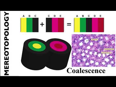
Coalescence
A coalescence creates a fusion situation where two or more lyphs are treated as being a single entity.
There are two types of coalescence, both describing material fusion. In both cases, coalescence can only occur between lyphs that have exactly the same material composition:
Connecting coalescencerepresents a ‘sideways’ connection between two or more lyphs such that their outermost layer is shared between them. The visualisation of such a situation requires that only a "single" depiction of these layers is shown. Technically, we still use two visual objects which, however, are aligned in such a way that they appear as a single object (provided that they are of the same size).Embedding coalescencerepresents dropping of a contained lyph into a container lyph such that the outer layer of the contained lyph fuses with the container lyph. The visualisation of such a situation requires that only the container lyph is shown.
The Coalescence class, apart from the generic resource properties id, name, etc., defines fields topology and lyphs which the model author should use to specify the type of the coalescence, CONNECTING or EMBEDDING (default value is CONNECTING) and the coalescing lyphs, respectively. The field lyphs expects an array of coalescing lyphs. Although semantically the order of the lyphs in the connecting coalescence are not important, in the viewer, the first lyph is treated as a "master" - while connecting the graphical depictions of coalescing lyphs, all subsequent lyphs are pushed by the force-directed layout to approach the "master" lyph and realign their outermost layers to match the outermost layer of the first lyph. In the case of the embedded coalescence, the first lyph is expected to be the housing lyph.
If a coalescence resource is defined on abstract lyphs (lyph templates), it is considered abstract and works as a template to generate coalescences among lyphs that inherit the abstract lyphs.
The images below show the visualization of connecting coalescence: two coalescing lyphs, Visceral Bowman's capsule and Glomerulus, share a common outer layer, Basement membrane:

In the case of embedding coalescence, the outer layer of the embedded lyph blends with the layer of the housing lyph, we make it invisible:

Group
A group is a subset of entities from the ApiNATOMY model (which can also be seen as a group) that have a common semantic meaning and/or a distinct set of visual characteristics. A group can include nodes, links, lyphs, materials, and other groups (subgroups) via the properties with the corresponding names.
In the example below, we define a group of blood vessels by joining two subgroups, arterial and venous vessels.
    "groups": [
        {
          "id"    : "omega",
          "name"  : "Blood vessels",
          "groups": ["arterial", "venous"]
        },
        {
          "id"    : "arterial",
          "name"  : "Arterial",
          "nodes" : [ "nLR00", "nLR01", "nLR02", "nLR03", "nLR04", "nLR05" ],
          "links" : [ "LR00", "LR01", "LR02", "LR03", "LR04" ]
        },
        {
          "id"    : "venous",
          "name"  : "Venous",
          "nodes" : [ "nLR10", "nLR11", "nLR12", "nLR13", "nLR14", "nLR15", "nLR16" ],
          "links" : [ "LR10", "LR11", "LR12", "LR13", "LR14", "LR15" ]
        }
    ]
Resource visibility rules
Since ApiNATOMY models typically consist of numerous resources, visualizing all of them at the same time in the graph view is infeasible. Therefore, a set of resource visibility rules apply on graph vertices, edges, and lyphs. In the most trivial case, only resources included to visible groups are shown on the screen. Group visibility is controlled via checkbox controls at the Control Panel. However, group resources may have relationship dependencies affecting their visibility. Moreover, for generated groups, a set of implicit inclusion rules applies. Finally, various groups may include overlapping sets of resources or subgroups with conflicting visibility settings.
Regarding relationship-based constraints, the following visibility rules apply:
- A graph edge (connectivity model link or scaffold wire) is visible if it is included to a visible group and its source and target ends are also visible.
- An edge that lies on a border is visible if the border is visible. The border is visible if its hosting shape (lyph or region) is visible.
- A lyph is visible if a link it conveys is visible or it is a layer in a visible lyph.
Generated groups
When expanding group templates such as chains, implicitly declared groups are generated. Such groups can be recognized by its properties "generated" set to True and "generatedFrom" pointing to the template that provides rules for the group resource inclusion.
If a generated group includes a link, the following resources are also included to the group:
- its conveying lyph,
- its source and target ends,
- its hosted nodes.
If a generated group includes a lyph, the following resources are also included to the group:
- its layer lyphs,
- its internal lyphs,
- its internal nodes.
If a generated group includes a node, the following resources are also included to the group:
- its clone nodes (copies of the node hosted by adjacent lyphs or their borders)
- collapsible links that have the node as one of its ends.
Note that if someone wants to hide or show a subgraph, it is not necessary to list lyphs conveyed by the graph links, the lyphs are considered part of the link definition for that purpose. However, if one wants to be able to toggle a certain set of lyphs but not their axes, the lyphs should be included to some group explicitly.
Dynamic groups
The viewer automatically analyzes an input model and creates dynamic groups with closed flow, i.e.,
sub-graphs topologically equivalent to a CYST. Such components are important and may represent anatomically meaningful
systems such as neurons and neuron parts. The algorithm places discovered groups under the title Dynamic groups.
A modeller can assign a meaningful name to a dynamic group by defining an empty group, i.e.,
{"id": "neuron-8", "name": "Neuron 8"}
and pointing any lyph from this group to it via property seedIn, i.e.,
   {
     "id": "snl18",
     "name": "Soma of SPR neuron in L1_Neuron 8 (kblad)",
     "seedIn": "neuron-8"
   }
Graph
Graph is the top-level group that in addition to all the group parameters contains a config object. The field is not part of the semantic physiology model but it can be used to define user preferences regarding the visualization of a certain model. For example, a field filter within this object is currently used to exclude resources with given identifiers from appearing in the relationship graph.
"config": {
    "filter": ["6", "11", "12", "14", "15", "16", "17", "20", "21"]
}
Among other properties that can be stated here are the default label fields.
Group templates
Group template is a generic concept to encapsulate resource definitions that result into automatic generation of subgraphs with certain structure and/or semantic meaning. A distinct property of the resource objects of this type is a readonly group property that establishes the relationship between the template and the generated group.
Another currently supported property of this generic class is length that sets in percentage the desired length of the maximal path in the generated group. This property is used to compute the default link length and, consequently, control the size of the lyph shape conveyed by the link.
There is ongoing work on supporting visual resource styles that one will be able to refer to from groups or group templates to define the appearance of links, lyphs and nodes in the entire (auto-generated) group.
Chain
This template instructs the model generator to create a chain from an ordered list of lyphs, i.e., a linear concatenation of advective edges that convey the material of the innermost layer of these conveying lyphs. This requires the lyphs in the ordered list to have their innermost layers constituted of the same material.
The listing below shows an example of chain template definition:
{
  "id": "c1",
  "lyphs": ["200", "203", "204", "205", "206", "207", "208", "209", "210", "211", "212", "213", "214", "215", "216"],
  "root": "s",
  "leaf": "t"
}
Apart from the list of lyphs, the template includes root and leaf properties
to name the source and the target nodes of the chain.
They are helpful to integrate the chain as a fragment into a larger model graph.
If the root is not explicitly defined, an error message is issued (an artificial node is created to
visualize the chain, but semantically such model is likely to be incorrect and has to be revised by the author).
Alternatively, instead of providing of lyphs to connect to a chain, a modeller can provide an abstract lyph
via the property lyphTemplate and indicate the number of levels in a generated chain via the property
numLevels. For example, the template below will generate a chain of 5 levels conveyed by identical lyphs with 3 layers:
{
    "chains": [
       {
         "id": "axonal",
         "name": "Axonal omega tree",
         "root": "a",
         "numLevels": 5,
         "lyphTemplate": "neuronBag"
       }
     ],
    "lyphs": [
       {
         "id": "neuronBag",
         "isTemplate": true,
         "topology": "BAG",
         "layers": ["cytosol", "plasma", "fluid"]
       }
     ]
}
Yet another option to define (or customize a chain), is to use property levels that accepts link references (
or partial specifications):
{
  "id"          : "c1",
  "root"        : "a",
  "levels"      : [
    {"source": "a", "target": "b", "conveyingLyph": "lyph1"},
    {"source": "b", "target": "c", "conveyingLyph": "lyph2"},
    {"source": "c", "target": "d", "conveyingLyph": "lyph3"},
    {"source": "d", "target": "e", "conveyingLyph": "lyph4"},
    {"source": "e", "target": "f", "conveyingLyph": "lyph5"}
  ]
}
Note that if numLevels and lyphTemplate are provided, they can be used to generate default levels which then
can be replaced by specified links via the levels field. For example, if one wants to define a chain with 5 levels conveyed by identical lyphs,
and replace 3rd level with another lyph, only the 3rd level link can be provided:
{
    "id"           : "c1",
    "root"         : "a",
    "numLevels"    : 5,
    "lyphTemplate" : "neuronBag",
    "levels"       : [{}, {}, {"conveyingLyph": "lyph3"}, {}, {}]
}
Since it may be tedious for modelers to specify all levels via defining links
(i.e., defining source and target nodes, connected links, and conveying lyphs at each level),
for Excel spreadsheets we provide a syntactic sugar to simplify definition of chains
passing via given nodes. This is done via the levelTargets property that expects a string with pairs
of level index followed by a corresponding level target node, i.e., spreadsheet field 0:n1,3:n3,5:n5
is a shorthand notation for
"levels" : [ {"target": "n1"},{},{"target": "n3"},{},{"target": "n5"}]
It is sufficient to indicate only level target nodes as this does not cover only the start node of the
first level which is expected in the chain's root property.
Yet another common variant of chain definition is via housingLyphs or housingChain properties.
The former is used list a set of lyphs that house the chain, the latter expects a reference to another chain whose
level lyphs house the chain.
{
  "id"          : "c1",
  "root"        : "a",
  "lyphTemplate": "lyph",
  "housingLyphs": ["lyph1", "lyph2", "lyph3", "lyph4"]
}
If a housingChain reference is used, it is possible to indicate the index range to
define the part of the housing chain that houses the current chain lyphs. Moreover,
if the housing chain is generated, and the identifiers of layers are not available, the housingLayers property can be
used to refer to the indices of the layers in housing lyphs that embed the chain levels.
{
  "id"           : "t1",
  "root"         : "n1",
  "leaf"         : "n2",
  "lyphTemplate" : "229",
  "housingChain" : "c1",
  "housingRange" : {"min": 0, "max": 7},
  "housingLayers": [6,3,4,6,6,6,6]
}

Tree
Branching underlies the formation of numerous body systems, including the nervous system, the respiratory system, many internal glands, and the vasculature. An omega tree is a template to create a rooted tree data structure (a graph in which any two vertices are connected by exactly one path, and one node is designated the root) that we use in ApiNATOMY to model branching systems.
The Tree resource class allows users to specify a root of the tree via an optional property root that can point into an existing node. If the root node is not specified, it is either automatically generated or assigned to coincide with the source node of a link that represents the first level of the tree.
We define the level of a tree branch as the number of edges between the target node of the link and the root. A user may specify the required number of levels in a tree via its optional property numLevels which expects a positive integer value. Given the desired number of levels, the ApiNATOMY lyph viewer can generate a group (a read-only property that refers to a Group resource and encompasses all necessary nodes and links) to represent the tree. If the property lyphTemplate points to an abstract lyph, the generated links for each tree level then convey lyphs which are subtypes of this template.
Alternatively, the tree branches can be specified, partially or fully, via the property levels which expects an array of partial or complete link definitions corresponding to the tree levels. If this array contains an empty object, the missing tree level branch is auto-generated. If instead it points to an existing link, the corresponding link then becomes the branch of the tree. If source, target, or both ends of the link resource are not specified, they are auto-generated. Otherwise, it is expected that incident links (connected tree branches) share a common node; the tool will issue a warning if this is not the case.
"trees": [
    {
         "id"          : "axonal",
         "name"        : "Axonal omega tree",
         "root"        : "a",
         "numLevels"   : 5,
         "lyphTemplate": "neuronBag"
    },
    {
         "id"          : "UOT",
         "name"        : "Urinary Omega Tree",
         "root"        : "b",
         "levels"      : ["lnk1", "lnk2", "lnk3", "lnk4", "lnk5", "lnk6", "lnk7", "lnk8", "lnk9", "lnk10",
            "lnk11", "lnk12", "lnk13", "lnk14", "lnk15", "lnk16", "lnk17", "lnk18", "lnk19", "lnk20", "lnk21"],
         "branchingFactors": [1, 1, 2, 1, 1, 1, 3, 3, 20, 8, 9, 8, 9]
    }
]
Our examples section demonstrates in full detail how to define omega trees using both lyphTemplate and levels properties. A combination of both approaches may help modellers to reduce an effort while specifying multi-level trees where the majority of the branches convey the same lyphs (involve the same tissue structures) while certain levels either convey different lyphs or are characterized by unique features that need to be modelled in a special way.
The trees defined this way actually do not have any branching, they look like liner chains of enumerated links. We refer to such trees as canonical, meaning that they define the basic structure necessary to generate a branching tree that models an organ or a physiological subsystem. The branching can happen at each level of the canonical tree definition, and the number of branches per level can be specified in the branchingFactors array. The size of the array does not need to coincide with the size of the levels array - branching stops at the last level with branching factor greater than 1.
A user may define a required number of branching tree instances produced from the canonical tree specification. This is done with the help of the boolean property numInstances. The generated subgraphs representing branching tree instances are available via the read-only property instances in the expanded ApiNATOMY model. The lyphs for a tree instance are assigned create3d property, i.e., the generated tree instance can be visualized using solid 3d lyph renderings.
In the case of trees with branches that convey lyphs derived from a common lyphTemplate pattern, we can use the topology property of the lyph template to define the overall topology of the tree.
Generally, lyphs originating from a lyph template inherit its topology. However, the lyphs conveyed by the tree edges work as a single conduit with topological borders at the start and the end levels (root and leaves) of the tree compliant with the borders of the lyph template. Thus, the topology of the lyphs on tree edges is defined according to the table below:
| Lyph template | Radial borders | Tree | Level 1 | Levels 2..N-1 | Level N |
|---|---|---|---|---|---|
| TUBE | both open | TUBE | TUBE | TUBE | TUBE |
| BAG | 1st closed | BAG | TUBE | TUBE | BAG |
| BAG2 | 2nd closed | BAG2 | BAG2 | TUBE | TUBE |
| CYST | both closed | CYST | BAG2 | TUBE | BAG |
A tree template can be used to reduce repetition and possibility of error by automating the creation of a tree and associated conveying lyphs to distribute/embed conveying lyphs over an ordered list of housing lyphs. If the housingLyphs list is provided in a tree template, the number of levels is set to equal the size of this list, and a tree group with no branching is generated, then each level of the generated tree is bundled with the corresponding housing lyph as follows:
- The edges for the non-terminal housing lyphs span the housing lyph completely. The nodes of these edges anchor on the radial borders of the outermost layer of the housing lyph, i.e. they run parallel to the longitudinal borders. For the first and the last lyphs in the
housingLyphsset, only one node anchors on the radial border, the other "hangs free" inside the housing lyph. - The housing lyph is bundled with the tree level via its property
bundles. Respectively, the level link refers to the housing lyph via its propertyfasciculatesIn - Finally, the embedded coalescence resource is created to link the housing lyph and the lyph conveyed by the bundled link.
The fragment below shows an example of housed tree definition. More details about this model can be found in the Examples section (Bolser-Lewis map)
{
  "id": "t1",
  "name": "Neuron",
  "lyphTemplate": "229",
  "housingLyphs": ["202", "201", "200", "203", "204", "205", "206", "207", "208", "209", "210", "211", "212", "213", "214", "228"]
}
The image below shows a neuron tree aligned along the chain of housing lyphs.

Semantically, lyphs in contiguous chains of lyphs have a common border, but because the chosen ApiNATOMY visualization approach depicts lyphs as centered icons with separate borders, the alignment of an omega tree that respects the border constraints set by the rules above requires the non-terminal level link ends to be placed on two separate lines. To address this problem, we rely on the node clones and collapsible links (drawn as dashed lines) that connect two copies of the same node. Developers who plan to work with the ApiNATOMY models should keep this in mind when traversing the ApiNATOMY graph - two semantically adjacent graph links can be separated by an auxiliary collapsible link that does not convey any lyphs. Hence, to access a link that models the next level in the generated tree group, starting from the tree level link L1,one may need to use the following 3 step traversals:
L1.target.clones[0].sourceOf => L2
Here, L1.target gives the target node of L1, then clones[0] field gives a reference to its clone (there can be more clones of the same node as this mechanism is not limited by the canonical tree level alignment), and, finally, sourceOf field would provide the following link, L2.
For the transition in the reverse direction, the similar path can be used via the opposite cloneOf field that links the cloned node to its prototype:
L2.source.cloneOf.targetOf => L1
Channel
The Channel resource class provides fields to define a template that will instruct the model generator to create specialized assemblies (groups, subgraphs) that represent membrane channels incorporated into the given housing lyphs.
To create membrane channel components, a model author provides:
- an identifier for the channel alone with optional characteristics shared by all ApiNATOMY resources, i.e., name, external annotations, etc.;
- identifiers of housing lyphs. A
housing lyphis a lyph of at least three layers representing some cell or organelle (e.g. Sarcoplasmic Reticulum) such that the middle layer of this lyph is a membrane; - the material payload that is conveyed by the diffusive edge;
The identifiers of the housing lyphs and materials conveyed by the diffusive edges of the channel are specified in the resource properties housingLyphs and materials, respectively.
Alternatively, a lyph can refer to the channel it houses via its property channel.
Given these data, the model generator creates three tube lyphs representing the three segments of the membrane channel (MC): internal, membranous and external. Each of the MC segments consists of three layers as follows:
- innermost, or the content;
- middle, or the wall;
- outermost, or the same
stuff(material) as the lyph that contains it; The group assembly generated given such a template will include 23 resources (4 nodes, 3 links, 3 lyphs with 3 layers each, 3 coalescences, and a group resource that encompasses nodes, links and lyphs of the channel instance). If the housing lyph is a template, this number of resources is then replicated for each channel instance housed by a lyph instance that is a subtype of the template.
The three MC segments are placed (housed) respectively in:
- the innermost layer of the housing lyph;
- the second layer of the housing lyph, which must be constituted of material of type membrane
- the third layer of the housing lyph. To fulfill this requirement, we automatically set constraints that require channel nodes to be hosted by the borders of the layers of the housing lyph.
The third layer of each MC segment undergoes an embedding coalescence with the layer of the housing lyph that contains it.
Each of the three MC segments conveys a diffusive edge such that both nodes of the edge conveyed by the MC segment in the second (membranous) layer are shared by the other two diffusive edges.
Diffusive edges are associated with the links that convey the membrane channels (i.e., the link's conveyingType is set to DIFFUSIVE) and the material in the channel object is copied to the conveyingMaterials property of the link.
The images below show two membrane channels, mc1: Na-Ca exchanger and mc2: SR Ca-ATPase, which are housed by the abstract lyphs (templates) with IDs 63 and 60: Myocyte and Sarcoplasmic reticulum, respectively.
The first image shows abstract assemblies, the second image shows the instances of these assemblies housed by two lyph instances derived from the abstract Myocyte and Sarcoplasmic reticulum lyph templates.


As one can see, channels are defined in a minimalistic way, but may cause the model generator to automatically create a potentially large number of resources, the modeller should keep this in mind to avoid state space explosion.
Scaffold model
Anchor
Anchors are graph vertices that help to position and shape connectivity model parts.
An anchor represents a vertice and its class Anchor extends the generic class Vertice, similarly to
the class Node in the connectivity model. Two of basic properties in an anchor object definition
are sourceOf and targetOf which point to the wires incoming to and outgoing from this anchor.
A boolean property cardinal can be used to mark important anchors that have special positioning
constraints in scaffold models such as Too-map.
Analogously to nodes, the position of an anchor is defined via the layout property. However, anchor coordinates
are 2-dimensional:
{
 "anchors": [
  {
   "id": "L",
   "name": "LUNG CAPILLARY",
   "cardinal": true,
   "layout": {
    "x": 90,
    "y": -10
   },
   "color": "#FF0000"
  }
 ]
}
An anchor can also be bound to a wire via the properties hostedBy that provides a reference to a wire and
offset that specifies the offset in percentage from the start of the wire.
Placing an anchor to the area occupied by a region is done via its field internalIn.
If an anchor resource is used as part of region definition in region's property borderAnchors,
it will supply an auto-assigned read-only property onBorderInRegion.
Another read-only property partOf indicates to which scaffold the anchor belongs.
A connectivity model node bound to an anchor can be retrieved via the anchor's property anchoredNode.
Wire
Wires are graph edges that help to position and shape connectivity model parts.
Since a wire represents an edge and its class Wire extends the generic class Edge similarly to links,
two of its fundamental properties are source and target that point to the edge source and target
vertices (anchors). Unlike links, wires do not convey lyphs.
An important property that defines the shape of the wire is geometry. It can take the same values as
link's geometry, namely, link | arc| spline | invisible | semicircle | rectangle, and, in addition,
ellipse, which defines an elliptic curve without source or target.
For elliptic wires, property radius is used to set its x-radius and y-radius:
{
  "id"       : "ellipticWire",
  "geometry" : "ellipse",
  "radius"   : {"x": 100, "y": 80}
}
The shape of spline wires can be additionally controlled by the property controlPoint which sets a control point for
the cubic Bézier curve. The shape of the arc or spline wires can be adjusted using the curvature parameter
which defines the curvature of an arc or spline edge, as percentage of its length.
Curvature is used to compute a control point for dynamic edges (i.e., edges with ends whose position depends
on other elements, this applies to the links as well).
Analogously to hostedNodes for links, the wire has the field hostedAnchors which lists anchors located on
the wire. It also has an automatically assigned (read-only) property facetIn to find regions for which the wire serves as a facet.
Another read-only property partOf indicates to which scaffold the wire belongs.
The main use of wires in ApiNATOMY models is to define trajectories for chains. The wire's property
wiredChains shows which chains get governed by the wire.
Region
Regions are flat shapes that help to provide context to the model, e.d., by placing certain process graphs into a region named "Lungs", one can indicate that this process is happening in the lungs. Region internal content is similar to the content of a lyph. Regions are static and their positions are given in 2D coordinates. The border of the region can include any number of straight segments (links), unlike lyphs which always have 4 sides.
{
 "regions": [
  {
   "id"     : "cs",
   "name"   : "Cardiac system",
   "points" : [{"x": -75, "y": 20}, {"x": -75, "y": 75},{"x": -25, "y": 75},{"x": -25, "y": 20}],
   "color"  : "#fbb03f"
  },
  {
   "id"     : "cns",
   "name"   : "Central Nervous System",
   "points" : [{"x": -65, "y": -50}, {"x": -65, "y": -15}, {"x": 65, "y": -15}, {"x": 65, "y": -50}],
   "color"  : "#f4ed2f"
  }
 ]
}
Component
A component is part of the scaffold that is similar to a group in the connectivity model.
A component includes aggregating fields for defining or referring to its resources: anchors, wires, regions, and nested components.
TOO Map
The TOO map provides the ApiNATOMY author with a wireframe schematic of the body to overview and quality-check connectivity. See video. This subway-style whole-body map depicts as a topological scaffold the three main flow thoroughfares of extracellular material: in blue, a 'T'-shaped depiction of CerebroSpinal Fluid (CSF), in red an inner 'O'-shape denotes the circulation of blood, and in green the outer 'O'-shape denotes the flow of materials on the surface of the body, such as digestive juices, food, chyme, chyle, faeces, air, sweat, tears, mucus, urine, milk, reproductive fluids and products of conception. (Hence: 'T' + 'O' + 'O' = TOO). Stylistically revisits a historical technique in map making known as the T-and-O map.
The images below show the scaffold mock-up and ApiNATOMY rendering:


Connectivity model + scaffold:
A node can be bound to a scaffold's anchor via its propertyanchoredTo.
To make a chain stretch along a given wire, place the reference to the wire to the chain's property wiredTo.
By default, a wired chain gets its root anchored to the source of the wire, and it's leaf to the target of the wire.
The directionality can be reversed if a Boolean chain's property startFromLeaf is set to true.
Note that the intermediate nodes of a wired chain directly follow the trajectory of the wire while
the intermediate nodes of a chain with just root and leaf nodes anchored to a wire ends are governed by
the forced-directed layout algorithm.
Lyphs and groups of lyphs can be placed to the area of a scaffold region via their property hostedBy.
The image below shows an example of a rendering for a connectivity model with nodes and chains bound to the anchors and wires of the TOO map.

Examples
Basal Ganglia
The basal ganglia are a group of subcortical nuclei at the base of the forebrain and top of the midbrain. The basal ganglia are associated with a variety of functions, including control of voluntary motor movements, procedural learning, habit learning, eye movements, cognition, and emotion. Basal ganglia are strongly interconnected with the cerebral cortex, thalamus, and brainstem, as well as several other brain areas.

The ApiNATOMY model automatically reproduces the layout from the schematic representation of the basal ganglia created by the physiology experts, given relational constraints among its constituent parts. Conceptually, the model consists of:
- 4 context lyphs: Basal Ganglia, Putamen, Globus Pallidus external (GPe) and Globus Pallidus internal (GPi) segments;
- a model of a neuron composed of 3 parts:
dendriteandaxonmodelled as trees (we call themomega trees) and a conduit representing the axonhillock(a specialized part of the cell body, or soma, of a neuron that connects to the axon) that joins the omega trees on its sides.

Even though omega trees often look like simple chains in our schematics, the underlying data model implies that a branching tree can be generated from the canonical representation given model parameters such as branching factor or mean number of branches at each level).
Technically, the model is essentially a JSON file with 4 fields: nodes, links, lyphs, and trees. The context lyphs, Putamen, GPe and GPi, are modelled as internal lyphs of Basal Ganglia:
   {
      "id"    : "bg",
      "name"  : "Basal Ganglia",
      "color" : "#d1d2d4",
      "internalLyphColumns": 3,
      "internalLyphs": [ "putamen", "gpe", "gpi" ]
   }
This means that they are positioned on a grid within their container lyph, and the corresponding parameter, internalLyphColumns: 3 indicates that the grid should contain 3 columns. The number
of rows depends on the number of internal lyphs within the container.
Other space allocation methods for internal lyphs will be supported upon demand, for example,
template-based treemaps appear to be particularly useful if we need to dedicate areas of various size to internal lyphs while preserving relevant adjacency constraints.
The nodes and links to model rotational axes of internal lyphs are auto generated (they can also be defined explicitly if a user wants to override the default properties, i.e., make them visible, or specify relationships between them and other graph entities). Thus, in our model, we only define the position and the size of the main context lyph's axis, Basal Ganglia:
    "nodes": [
        { "id": "a", "layout": {"x": -100, "y": 100, "z": 0 } },
        { "id": "b", "layout": { "x": 100, "y": 100, "z": 0 } },...
    ],
    "links": [
        {
            "id"      : "main",
            "source"  : "a",
            "target"  : "b",
            "length"  : 100,
            "geometry": "invisible",
            "conveyingLyph": "bg"
        },...
    ]
The trees property is an array with 2 objects defining the dendrite 1-level tree and the axonal 5-level trees:
    "trees": [
        {
          "id"          : "dendrite",
          "name"        : "Dendrite omega tree",
          "root"        : "n1",
          "numLevels"   : 1,
          "lyphTemplate": "neuronBag"
        },
        {
          "id"          : "axonal",
          "name"        : "Axonal omega tree",
          "root"        : "n2",
          "numLevels"   : 5,
          "lyphTemplate": "neuronBag"
        }
    ],
The tree root nodes are named n1 and n2, these names are explicitly given while defining the the axis of the axon hillock, and by referring to them in the tree model, we indicate that the roots of the axonal and dendrite trees coincide with the ends of the hillock.
Similarly to the root nodes, it is possible to plug an external link, a node or a lyph into the generated tree at a certain level via the optional levels property which expects an array with (partial) link definitions (see JSON Schema definition of the tree model for more details).
In the current model, we do not refer to external entities while defining the content of the tree branches. However, all auto-generated ApiNATOMY entities are also assigned IDs that can be referenced later to connect the part of the graph obtained from the tree template with the rest of the model. The identifies for auto-generated tree parts are formed using the following patterns:
{$tree.id}_node{$index}{$tree.id}_lnk{$index}{$tree.id}_lyph{$index}
where $tree.id is the identifier of the tree, and $index refers to a tree level.
For the node names, the $index ranges from 0 to N, where N is the number of levels. Hence,
the root node corresponds to the index = 0, the end node of the tree branch at the first level - to the index = 1, and so on. For the link and lyph names, the index ranges from 1 to N. For example, the valid ID names for the basal ganglia trees:
axonal_node3- end node of the 3d level of the 'axonal' treeaxonal_lyph5- lyph at the 5th level of the 'axonal' tree,dendrite_lnk1- link at the 1st level of the 'dendrite' tree.
These names can be used to impose positional constraints on the generated entities. For example, in our model, the axonal tree node is located on the 2nd radial border of the GPi lyph, while two axonal tree level lyphs are hosted by (mapped to the surface of) the the GPi lyph.
    {
        "id"          : "gpi",
        "name"        : "GPi",
        "color"       : "#939598",
        "height"      : 30,
        "border"      : { "borders": [ {}, {}, {}, { "hostedNodes": [ "axonal_node3" ] }]},
        "hostedLyphs" : [ "axonal_lyph4", "axonal_lyph5" ]
    }
Another version of the basal ganglia shows how one can combine explicitly assigned tree levels with auto-generated ones.
The lyphTemplate field in these omega tree models refers to the lyph pattern to derive the structure of the conduits in the tree branches. Firstly, the tool expands the tree template by creating the necessary graph structure (a rooted tree with the required number of levels). Secondly, the blank lyph definitions associated with the tree graph are added to the subtypes property of the lyph template. At the next stage, the lyph viewer will process the lyph templates: the prototype lyph layers, color and size settings are copied to all template subtypes.
Hence, at the tree expansion stage, the user definition of the template lyph:
    "lyphs": [
        {
            "id"        : "neuronBag",
            "isTemplate": true,
            "topology"  : "BAG",
            "color"     : "#ccc",
            "scale": {
                "width" : 80,
                "height": 80
            },
            "layers": ["cytosol", "plasma", "fluid"]
        },...
    ]
is extended with the definition of subtype lyphs which will get 3 layers and will occupy each the square area with a side length computed as 80% of their axis length. Note that the hillock lyph also derives its structure from the neuronBag template, as indicated by its property supertype:
   {
        "id"       : "hillock",
        "name"     : "Hillock",
        "supertype": "neuronBag",
        "topology" : "TUBE"
   },
Hence, after the generation of entities to represent required tree structures and bi-directional relationship synchronization, the user definition of the neuron template in the model will be auto-completed, i.e., the lyph template will know all lyphs that replicated its layers via its subtypes property:
"subtypes": [axonal_lyph1,...,axonal_lyph5, dendrite_lyph1, hillock]
The lyphs conveyed by the tree edges are seen as a single conduit with topological borders at the start and the end levels (root and leaves) of the tree compliant with the borders of the lyph template. In our example, the lyph template is of type BAG. Hence, the conveying lyphs at the end levels, dendrite_lyph1 and axonal_lyph5, are of the type BAG while all the intermediate level lyphs, axonal_lyph1,...,axonal_lyph4, are of the type TUBE.
The topology of the hillock lyph, which also inherits the layer structure from the neuronBag lyph template, has to be explicitly defined as TUBE to override the inherited topology from the template.
The image below shows the layout created by the tool for the Basal Ganglia scenario based on the
resource definition explained in this section.

There is also an option to instruct the editor to generate 3d representation of lyphs: if a lyph's attribute create3d is set to true, the user will see 3d-dimensional lyphs when the option lyphs 3d in the control panel is enabled. When generating omega trees, the viewer automatically sets create3d to true, the corresponding layout for the Basal ganglia scenario is shown in the snapshot below.

The live demo of this scenario with the possibility to edit the model file in an integrated JSON editor is available here.
Urinary Omega Tree
This model illustrates the ApiNATOMY format for the urinary arborisation. The purpose of this example is to illustrate how one can model an omega tree with branching points and resource annotation with references to external ontologies.

The urinary tree model consists of 21 level. Levels are defined as links conveying specific lyphs, from Intravesical Urethra to Visceral Bowman's Capsule. The layer structure of these lyphs is modelled with the help of abstract templates that correspond to physiological tissues: urine (URN), transitional epithelium (TE), basement membrane (BM), muscosa (Mus), muscularis (Ms1) etc.
  {
      "id"        : "IU",
      "name"      : "Intravesical urethra",
      "topology"  : "TUBE",
      "length"    : {"min": 2, "max": 2},
      "thickness" : {"min": 3, "max": 3},
      "layers"    : ["URN", "Mcs", "Ms1"],
      "external"  : ["UBERON:0000057"]
  },
  {
      "id"        : "URN",
      "name"      : "Urine",
      "color"     : "#f9ed32",
      "isTemplate": true,
      "external"  : ["UBERON:0001088"]
  },
  ...
Whenever the specific lyphs refer to abstract lyphs as their layers, meaning that the conduit we model consists of certain tissues, the lyph viewer automatically generates lyph instances and replaces the conduit layers with the references to the generated lyphs representing tissues within the conduits, i.e., urine in the intravesical urethra. The generated lyphs will refer to the template via their supertype field and later inherit a set of template properties, namely,
color, scale, height, width, length, thickness, as well as the references in the fields external and materials.
In the ApiNATOMY data model, trees are templates that replicate the given lyph template to the requited number of levels. However, it may be useful to define some or all of the tree levels by referring to already existing links. This is the case when there is no common lyph template that applies to all tree levels or when the tree is part of the bigger models and its elements are connected to other parts of the graph.
The urinary omega tree below is defined in the aforementioned manner: its levels are composed of existing links that convey various lyphs. In principle, the same subgraph could be defined as a simple group, but the tree concept allows us to specify the branching patterns and automatically generate an instance of a canonical tree. The canonical omega tree is the minimal construct that is necessary to represent the structural composition of a certain organ or a physiology system, the tree instance is an actual arborisation that adheres to the structural, dimensional and branching patterns in the canonical tree. Due to certain degrees of freedom (probabilistic branching patterns, level dimension ranges, etc.) in the canonical trees, the tree instances we generate may vary.
  "trees" : [
    {
      "id"          : "UOT",
      "name"        : "Urinary Omega Tree",
      "root"        : "uot-a",
      "numLevels"   : 21,
      "levels"      : ["uot-lnk1", "uot-lnk2", "uot-lnk3", "uot-lnk4", "uot-lnk5", "uot-lnk6", "uot-lnk7", "uot-lnk8", "uot-lnk9", "uot-lnk10",
         "uot-lnk11", "uot-lnk12","uot-lnk13", "uot-lnk14", "uot-lnk15", "uot-lnk16", "uot-lnk17","uot-lnk18","uot-lnk19", "uot-lnk20", "uot-lnk21"
      ],
      "branchingFactors": [1, 1, 2, 1, 1, 1, 3],
      "comment": "Branching factors for the rest of the tree removed to avoid state explosion ... 3, 20, 8, 9, 8, 9, 1, 1, 1, 1, 1, 1, 1, 1"
    }
  ]
The images below show the canonical omega tree for the Urinary system model in 2d and 3d.


The next image shows the snapshot of the omega tree instance with branching in levels 3 and 7. The actual model of the urinary omega tree has more branching points, but due to the number of visual elements needed to represent the entire model (appr. 90 million), the viewer cannot handle all of them in the same view. If necessary, we recommend to explore different branching points separately by setting branching factor for other levels to 1.

In this model, several subgroups of items are annotated with a single ontology term. We can represent such a many-to-one mapping by defining and annotating subgroups. hence, in the ApiMATOMY model for this system, you can find subgroups defining a nephron and a loop of Henle, with the corresponding UBERON term IDs.
"groups": [
    {
      "id"      : "nephron",
      "name"    : "Nephron",
      "nodes"   : ["uot-m", "uot-n", "uot-o","uot-p","uot-q","uot-r","uot-s","uot-t","uot-u","uot-v"],
      "links"   : [ "uot-lnk13", "uot-lnk14", "uot-lnk15", "uot-lnk16", "uot-lnk17", "uot-lnk18", "uot-lnk19", "uot-lnk20", "uot-lnk21"],
      "lyphs"   : ["DCT", "FPofTAL", "DST", "ATL", "DTL", "PST", "PCT", "PBC", "VBC"],
      "external": ["UBERON:0001285"]
    },
    {
      "id"      : "henle",
      "name"    : "Loop of Henle",
      "nodes"   : ["uot-n","uot-o","uot-p","uot-q","uot-r"],
      "links"   : ["uot-lnk14", "uot-lnk15", "uot-lnk16", "uot-lnk17"],
      "lyphs"   : ["FPofTAL", "DST", "ATL", "DTL"],
      "external": ["UBERON:0001288"]
    }
]
To instruct the viewer to stretch the tree from left to right, we add layout constraints to the tree root and leaf nodes. We also rely on the assign property and JSON path expressions to customize the appearance of the nodes and lyphs: the nodes' color is set to red while the main conveying lyphs are set to the neutral grey color.
 "assign": [
    {
      "path" : "$.nodes[*]",
      "value": { "color" : "red"}
    },
    {
      "path"  : "$.links[*].conveyingLyph",
      "value" : { "color" : "#ccc" }
    }
  ]
Bolser-Lewis map
Please note that this example shows a rough work-in-progress model that demonstrates the use of modeling concepts rather than preserves the physiological accuracy!
The example is based on a mock-up for the Bolser-Lewis model

The model author defined the necessary resources in the Excel format. The image below shows the snapshot of the Excel template we developed as alternative to the text-based JSON format. The model from the Excel template can be exported as an .xlsx file and opened from the ApiNATOMY model viewer. The integrated converter translates the model to the JSON-based input format.

The model shows the neuron tree passing through a chain of body compartments. As a requirement, the author wanted to generate the chain given an ordered list of conveying lyphs:

The chain template shown in the image above produces a chain of connected links that convey the lyphs from the chain's conveyingLyphs property:

The neuron tree needs to be generated to match the number of housing lyphs:

The specification above does not set numLevels or levels fields; instead the size of the housingLyphs array here is used to determine the number of generated tree levels; each tree level is then "embedded" to the corresponding housing lyph. This implies that the tree level link ends are hosted by the housing lyph or, in case of layered lyphs, its outermost layer
(hostedBy relationship is set).

Moreover, an embedding coalescence is defined between the pairs of the housing lyphs and the conveying lyphs of the tree levels they house.
One can observe that the generated omega tree has collapsible "spacer" links. These links should disappear in the views that do not require the same node to appear in two different locations (i.e., on borders of adjacent lyphs which are displayed with a gap). The lyph viewer determines whether spacer link ends are constrained based on the visibility of the related resources.

Variance in species
Variance handling fields appear in the Settings panel after loading a model with a variance specification.
The image below gives an example of such a specification within the WBKG (Whole Body Knowledge Graph) ApiNATOMY model.
Lyphs are annotated with the help of the varianceSpecs field.

By default, we show the maximal possible chain. When a variance spec is enabled via the settings panel, a combobox allows
a user to select a clade. We mainly need to worry about the field presence set to the value absent.
When a clade is selected, lyphs annotated as absent will be excluded from the model.
The image below shows the clade options available in the comb0-box of the Variance tab within the Settings panel.

Screenshots below show the Infraventricular-csf-tract:
- full chain,
- NCBITAxon:9989 vs-not-rodent variance (lyph-L6-spinal-segment absent),
- NCBITaxon:9606 vs-not-human variance (lyph-L6-spinal-segment and lyph-T13-spinal-segment absent)


Model editors
Model editors allow users to define or modify existing ApiNATOMY models using a selected set of predefined GUI-based operations. Among other ways to define models are JSON code and Excel-style spreadsheets.
Important: To save model changes performed via model editors described below, press Apply changes button in the
right-side toolbar of the corresponding editor. If there were changes made, the button is marked with
a red star (*). After that the updated input model will be processed by the model generator and appear in the model
graph viewer (first tab called "Viewer"). Time delay is possible
at this stage, this is a potentially computationally expensive process if a model requires generating numerous resources
from templates, so we advise to use it after the (significant amount of) editing is done.
Material editor
The "Material editor" tab provides a GUI for defining materials and material-to-material and material-to-lyph relationships
in ApiNATOMY input models. The editor consists of a main view that displays a directed acyclic graph (DAG)
of material composition, and a property editing panel that allows users to edit properties of a selected material.
The view shows the material composition relationship as defined by the materials/materialIn properties
of materials (and lyphs which can be viewed as complex materials) in the input model.
To select a material, click on a graph node, it will be highlighted with a grey border around the material node.
The node's incoming and outgoing edges in the DAG will also be highlighted as thick grey lines. Properties
of the selected material can be viewed and revised via the property editing panel on the right. The right bottom panel
shows lyph definitions in which the selected material is used as layer.

On a double click the view is changed to a tree view with the selected material as its root. This view shows the composition hierarchy of the root material, i.e., which materials it is used in (nodes connected with pink links and arrows directed towards the selected material) and which materials it includes (nodes connected with black links and arrows directed away from the selected material).

Operations
CRUD (Create, Read, Update, and Delete) operations can be performed on selected materials using mouse right-click
menus. These operations are context-dependent - they are applied to a selected material.
Each applied operation is registered and can be reverted or repeated using Undo and Redo buttons on the right-side
vertical toolbar.
Material properties
All resources in ApiNATOMY data model, including Material, are derived from an abtract class Resource ## connectivity model
and inherit from it basic properties id, name, and ontologyTerms.
Editing of these properties is performed in the same way for all types of resources.
A correct resource definition should include properties id and name that are used to identify the purpose of the resource and
include it into the model graph by reference from other resources. One can edit these properties via the editing panel
present in Material editor as well as other resource editors (Lyph editor, Chain editor, and Coalescence editor).
When identifier is changed, all references to the selected resource are replaced to the new identifier. Identifies should comply to the ApiNATOMY schema,
i.e., should not contain spaces or start from a digit. A resource name usually reflects its physiological meaning. However, names can be ambiguous, so to properly specify a physiological
part represented by a resource, modellers should annotate it with appropriate ontology terms.
Several terms can be assigned to each resource, one can add and remove ontology annotations using a plus icon and icons with
trash bin next to the terms in a list.
Once an annotation is added, it has a generated temporary identifier that needs to be replaced with a proper term reference.
Such a reference typically consists of an ontology prefix followed by a semicolon separator, and a term identifier in the
chosen ontology, e.g., UBERON:0001898 for hypothalamus in the Uber-anatomy ontology,
or FMA:5875 for the white communicating ramus in the Foundational Model of Anatomy ontology.

Create new material
To create a new material, click right button on an empty space and select Add material. A new loose node with temporary
identifier and name will be added to the graph, one can rename and annotate it via the property editing panel.
The screenshot below shows the menu to add a new material.

Create a new relationship
To include a material into another material, select a parent node, find a child material in the search box and press add button below. The relationship link will be created and appear in the graph. It is important to note that lyph templates can be seen as composite materials and may be used as constituent parts of other materials too. Existing lyph templates can be added to the graph and linked with existing nodes in the same way as materials, via the search panel. To define new lyph templates, use the Lyph editor.
The screenshot below shows a material node "Cellular component of alveolar epithelium" linked to a newly created material "New material 1" which was added via the search panel in the right. Apart from this material, the selected node contains also 2 lyph templates as its sub-materials.

Delete relationship
To delete a specific relationship, right click on the corresponding edge and press "Delete relation".

Delete material, disconnect parents or children
Right click on a material node shows context menu which allows modellers to remove the node from the model, disconnect it from its parents or children.

Define as material or Define as lyph
If a material includes undefined resource, it is shown in the graph with grey node. To correct the model, a user should add an explicit definition for the referred resource by either creating a material or lyph template with the given identifier. The corresponding node will be updated and the color will change to green (material) or orange (lyph template).

Lyph editor
The "Lyph editor" tab provides a GUI for defining lyphs and lyph-to-lyph relationships in ApiNATOMY input models. The editor consists of 3 hierarchical trees, and a property editing panel.
The first tree view shows the list of declared lyphs arranged into hierarchy by the
sypertype/subtypes relationships. By clicking on the lyph identifier in this component, one selects
a lyph to inspect and modify. The second view shows the layers of the selected lyph defined by
layers/layerIn relationships. The third view shows internal lyphs of the selected lyph
defined by internalLyphs/internalIn relationships.

Users can identify lyphs that have layers and/or internal lyphs by presence of special icons next to the lyph name in the lyph view. For example, a selected lyph in the image below has both layers and internal lyphs.
![]()
Operations
CRUD (Create, Read, Update, and Delete) operations can be performed on selected lyphs using mouse right-click
menus. These operations are context-dependent - they are applied to a selected lyph in an active tree and vary depending
what tree is active. An active tree is highlighted by a grey border around the tree name. Each applied operation is registered and can be
reverted or repeated using Undo and Redo buttons on the right-side toolbar.
Some operations, namely, creation of new lyphs
and transition from one editing state to another (undo/redo) are performed via a vertical toolbar in the right
part of the viewer.
Lyph properties
Lyph definition panel extends the general resource definition panel with controls to define lyph's topology, indicate whether a lyph is a reusable template or a specific instance, and assign lyphs to hosting regions.

Delete definition
Unlike delete operations described below which are context dependent, Delete definition can be performed from any
tree and only removes the chosen lyph declaration. This may produce a model with undefined references which will trigger a warning in the ApiNATOMY model (the tool will generate
an artificial lyph to proceed with the visualization).
Define as material or Define as lyph
It may happen that a lyph refers to a resource in its subtypes, layers or internalLyphs arrays, but the referred
resource is not declared in the model. To be able to display such a reference graphically in the trees, we generate a
tree node that represents the reference but does not correspond to an actual resource declaration in the model, such node
can be recognized by its grey color. Two options will be given in the context menu for such nodes: Define as lyph and
Define as material, which generate a new lyph or material declaration with the given id, respectively. After that the color
of the corresponding tree node should change to the light orange for a lyph or light green for a material.
Lyphs and templates
Lyph templates are just lyphs with property isTemplate set to true and they are part of the lyph tree.
All operations applicable to lyphs also apply to lyph templates and they are defined just as normal lyphs.
However, a lyph template defines an abstract entity that can be referred multiple times from various other structures
in a model, each such reference is substituted by a generated lyph instance
with a unique id by the ApiNATOMY model generator.
More importantly for model editing, lyph templates are often reused in definitions of other lyphs via properties
supertype or subtypes. Lyph templates are shown in yellow as opposed to light orange for normal lyphs.
Create new lyph
To create a new lyph, press top button New lyph on the right-side toolbar. A new lyph with identifier
_newLyph# and name New lyph # where # is a numerical order of the created lyph is added to the lyphs array
of the current ApiNATOMY model. A corresponding node is created and added to the top of the lyph tree.

Delete lyph
To delete a lyph from the model, select a lyph in the main tree and click Delete in the context menu.

This operation not only removes the definition, but also clears all the references to the deleted lyph. For example,
the image below shows 2 code changes induced by the deletion of the lyph lt-PNS-ganglion: not only its
declaration is removed, but also the supertype reference of the lyph lt-ganglion-visceral-mural
is cleared. Instead, if one wants to just detach subtype from the supertype, operation Remove parent
should be applied

Note that the same menu button in Layers and Internal lyphs trees will not delete the chosen lyph definition,
it only detaches the lyph from the layers and internalLyphs arrays of the selected lyph (root of these trees), respectively.
Add subtype
To add a subtype to a selected lyph that inherits the lyph's properties and layers, right-click and select Add in the
context menu. By default, a new lyph is created (as described in the operation Create new lyph)
and included to the subtypes of the selected lyph. However, if one wants to include an existing lyph,
choose this lyph in the search box on the top of the Settings panel. The image below illustrates
this case: first, we select lyph-superior-cervical-ganglion in the search box, then click Add on the lyph lt-white-ramus
in the lyph tree, defining the supertype/subtypes relationship between them:

Note that if a material is selected in the search box, a warning "Cannot add a non-lyph resource as subtype" will be issued.
Remove subtypes
To clear all subtypes from a lyph, select Remove children in the main tree. This operation removes references from the
lyph's property subtypes, the corresponding lyphs will appear at the top level of the main tree. The menu option is not
available for lyphs with no subtypes.
Remove supertype
Lyphs with a supertype are located in a tree brunch under their supertype. To remove the supertype from a lyph,
press a right mouse button on it and select Remove parent. The lyph will disappear from the subtree and appear
at the top level of the main list. The menu option is not available for lyphs without a supertype.

Layers
One can identify lyphs with layers in the lyph tree by the icon with three bars. This icon may disapper if you delete all
layers or reappear if you add a layer toa lyph that previously had no layers. The number of layers in a lyph also affects
the upper bar limit in the related internal tree's fields internalLyphsInLayers.
Add layer
To add a layer to a lyph specification, select the lyph in the Layers tree and press Add in the right mouse button
context menu. The operation works similarly to the Add subtype operation: if a lyph is selected via the search box,
it is included to the layers array, otherwise a new lyph is created and included to the layers. Note that one may add
materials as layers. It is also allowed to add the same material or lyph template several times to define more than one layer
composed of a certain tissue. However, if a user tries to include a lyph from the supertype/subtype hierarchy as a layer,
the editor will display an error message "Cannot add a layer to this lyph: hierarchy or dependency conflict!".
If a selected lyph has a supertype with layers, i.e., it will inherit layers from its supertype, we show these layers in the Layer tree with a locker icon. It is not possible to add a layer to such a lyph, the same error as above will be triggered.

Delete layer (or remove layerIn)
To delete a layer from a selected lyph, right-click on the layer you want to delete and select Delete or Remove parent.
Both operations are equivalent: the first is seen from the point of view of editing the layer tree root while the second
removes the parent layerIn property from the layer itself.
If a selected lyph has a supertype with layers, i.e., it will inherit layers from its supertype, we show these layers in the Layer tree with a locker icon. Such layers cannot be deleted or rearranged, to modify them one must edit the layers of the supertype.
Remove layers
To remove all layers of a selected lyph, right-click on the lyph with layers in the layer tree and press Remove children.

This operation will not be available for lyphs without layers.
Move layer up/down
The order of layers in a lyph is important. The first layer defines the innermost tissue of the corresponding physiological
structure while the last layer defines the outermost tissue. To change positions of layers, right-click on a layer and
choose Move up or Move down.

Internal lyphs
Internal lyphs define internal constituent parts of a selected lyph. They can be positioned in the selected lyph or its layers. To place an internal lyph to a layer of the selected lyph, indicate the ordinal number of the layer next to the internal lyph node.
Re-assigning internal lyphs to layers
Very often lyphs in ApiNATOMY models are not explicitly defined but are generated from generic lyph templates.
Each generated lyph contains generated layers whose identifiers are unknown at the modelling stage.
If a modeller wants to specify internal structure of one or more of these layers, the only option is to refer to them by
indicating their order within the main lyph. This can be achieved by supplying layer indices next to the items in
the internal lyph list, implying that the corresponding lyph belongs to the layer with the index given index, where
0 refers to the innermost, closest to the axis, lyph. Thus, in the screenshot below, the internal lyph lyph-laryngeal-mechanoreceptors
belongs to the layer with index 1. This lyph will be derived from the abstract material
mat-temporary-laryngeal-wall.

Model authors can specify and/or modify the layer index using the number input box next to an internal lyph. The maximal value in this list is bounded by the actual number of layers the host will have, whether they are inherited from the template or defined explicitely.
Add internal
To add an internal lyph to a lyph specification, select the lyph in the Internal lyphs tree and press Add in the
right mouse button context menu. The operation works similarly to the Add subtype operation: if a lyph
is selected via the search box, it is included to the internalLyphs array, otherwise a new lyph is created and becomes
internal in the selected lyph. Note that one may add materials as internal lyphs. It is not allowed to add the same
material or lyph template several times. an error message "Cannot add this internal lyph to the selected lyph!" will
be issued.
Delete internal lyph (or Remove internalIn)
To delete an internal lyph from a selected lyph, right-click on the lyph you want to delete and select Delete or Remove parent.
Both operations are equivalent: the first is seen from the point of view of editing the internal lyph tree root while the second
removes the parent internalIn property from the lyph itself.
Remove internal lyphs
To remove all internal lyphs from a selected lyph, right-click on the root node in the internal lyph tree and press
Remove children.
Chain editor
The "Chain editor" tab provides a GUI for combining lyphs into chains - sequences of nodes and links conveying lyphs which are included into a global model graph by joining graph nodes or via more complex relationships with its other elements (e.g., a chain can be wired to a scaffold wire or hosted by a scaffold region). The ApiNATOMY model schema has several templates for defining chains and various ways to specify their positioning. However, the Chain editor currently supports only one template, most needed for the whole body knowledge graph (WBKG) chain definition: a chain is simply defined as an ordered list of lyph instances.
The editor consists of a main view that displays a list of existing (already defined in a model) chains. By clicking on the chain identifier in this list, a user selects a chain to inspect and modify, the second list is updated to show lyphs of the selected chains. Chain's properties are shown in the right-hand panel. By clicking on a lyph in the lyph view, modellers can inspect the structure of the selected lyph - its layers are listed under the property definition panel in the bottom right.

Chain editing operations are performed in the same way as the operations described in the chapter about the Lyph editor.
Coalescence editor
The "Coalescence editor" tab provides a GUI for defining sets of coalescing lyphs, i.e., lyphs with shared or connecting tissue layers that llow penetration of fluids.
The editor consists of a main view that displays a list of existing (already present in a model) coalescence definitions. By clicking on the coalescence identifier in this list, a user selects a coalescence to inspect and modify. The second list in the editor is updated to show lyphs in the selected coalescence. A correct coalescence definition includes at least 2 lyph instances.
The properties of the selected coalescence are shown in the right-hand panel. By clicking on a lyph in the lyph view, modellers can inspect the structure of the selected lyph - its layers are listed under the property definition panel in the bottom right.

Coalescence editing operations are performed in the same way as the operations described in the chapter about the Lyph editor.
Validation messages
The ApiNATOMY viewer allows users to create, edit, load and compose model specifications. Naturally, such specifications may be incomplete or obsolete. They may contain errors, inconsistencies, or conflicting definitions. It is not possible to prevent all errors with just syntactic JSON-schema-based validation. While creating resource map from serialized input model, the tool checks whether assumed constraints are satisfied and provides corresponding log messages that may help users to debug and fix the model.
Errors
CHAIN_LEVEL_ERROR           : `A mismatch between link ends found at level`,
CHAIN_LYPH_TEMPLATE_MISSING : "Failed to find the lyph template definition in the parent group",

COALESCENCE_NO_LYPH         : "Unable to access lyph for coalescence definition",

EXCEL_DATA_TYPE_UNKNOWN     : "Excel to JSON: failed to determine data type",
EXCEL_INVALID_COLUMN_NAME   : "Excel to JSON: invalid column name",
EXCEL_NO_COLUMN_NAME        : "Excel to JSON: no column name",
EXCEL_PROPERTY_UNKNOWN      : "Excel to JSON: unrecognized property",
EXCEL_WRONG_ASSIGN_VALUE    : "Excel to JSON: wrong assign value",

GROUP_NO_LINK_VALIDATE      : "Link has no validateProcess function. Possible cause - misclassified resource",
GROUP_TEMPLATE_NO_CLASS     : "Could not find class definition for the field",

RESOURCE_JSON_PATH_ERROR    : "Failed to process JSONPath assignment statement",
RESOURCE_NO_REL_CLASS       : "Related resource class is undefined",
RESOURCE_NO_REL_PROPERTY    : "Related property specification is not found in the expected class",
RESOURCE_NO_ABSTRACT_CLASS  : "An abstract relationship field expects a reference to an existing resource or 'class' field in its value definition",
REF_UNDEFINED               : "Remaining references to undefined resources"
Warnings
 AUTO_GEN                    : "Auto-created missing resources",
 AUTO_GEN_EXTERNAL           : "Auto-created missing external resources",

 CHAIN_CONFLICT              : `Conflicting chain specification: both "housingLyphs" and "housingChain" are given. Proceeding with "housingLyphs"`,
 CHAIN_CONFLICT2             : `Conflicting chain specification: both "lyphs" and "levels" arrays are given. Proceeding with "lyphs"`,
 CHAIN_CONFLICT3             : `Conflicting specification of housing layer: layer's bundlesChains} property disagrees with the chain's housingLayers} property`,
 CHAIN_HOUSING_TEMPLATE      : "Housing lyph or its layer is a template",
 CHAIN_MAT_DIFF              : "Incorrectly defined chain pattern - innermost layers do not convey the same material",
 CHAIN_NO_COALESCENCE        : "Skipped a coalescence between a housing lyph and a conveying lyph of the chain level it bundles: the conveying lyph is not defined",
 CHAIN_NO_HOUSING            : `Incorrect chain specification: "housingChain" not found!`,
 CHAIN_NO_HOUSING_LYPH       : "Failed to find chain level housing lyph",
 CHAIN_NO_HOUSING_LAYERS     : "Failed to find all layers of the housing lyph",
 CHAIN_SKIPPED               : `Skipped faulty chain template. A correct chain template must have one of the following conditions met:
                                 (1) "numLevels" set to a positive number and non-empty "lyphTemplate",\n
                                 (2) non-empty list of "lyphs" to join to a chain,\n
                                 (3) non-empty list of "levels" which are (partially defined) links to join to a chain,\n
                                 (4) non-empty list of "housingLyphs",\n
                                 (5) non-empty "housingChain" reference with optional "housingRange" parameter`,
 CHAIN_UNDEFINED             : "Cannot expand undefined chain template",

 CHANNEL_NO_GROUP            : "Cannot create channel instances: canonical group not found",
 CHANNEL_NO_ID               : "Skipped channel template - it must have (non-empty) identifier",
 CHANNEL_NO_HOUSING_LYPH     : "Failed to find channel housing lyph",
 CHANNEL_NO_HOUSING_LAYER    : "Failed to find channel housing lyph layer",
 CHANNEL_NO_NODE             : "Failed to find channel group node",
 CHANNEL_UNDEFINED           : "Cannot expand undefined channel template",
 CHANNEL_VALIDATION_SKIPPED  : "Skipped validation of channel housing lyph: failed to find membrane lyph or material (GO:0016020)",
 CHANNEL_WRONG_LAYER         : "Second layer of the housing lyph is not a (subtype of) membrane (GO:0016020)",
 CHANNEL_WRONG_NUM_LAYERS    : "The number of layers in the housing lyph does not match the number of links in its membrane channel",

 COALESCENCE_NO_AXIS         : "A coalescing lyph is missing an axis",
 COALESCENCE_NO_INSTANCE     : "No lyph instances found for abstract coalescence",
 COALESCENCE_SELF            : "A lyph coalesces with itself or its layers",

 COMPONENT_SELF              : "The model contains self-references or cyclic component dependencies",

 EXCEL_NO_CLASS_NAME         : "Excel to JSON: class name not found",

 GROUP_GEN_NOT_EMPTY         : "Generated group already contains resources",
 GRAPH_LYPH_NO_AXIS          : "Failed to compute axis length for an internal lyph: axis undefined",
 GROUP_SELF                  : "The model contains self-references or cyclic group dependencies",

 LYPH_INTERNAL_NO_LAYER      : "Failed to locate layer lyph to reposition internal lyphs",
 LYPH_INTERNAL_OUT_RANGE     : "Failed to relocate internal lyph to layer: layer index out of range",
 LYPH_NO_TEMPLATE_LAYER      : "Template layer object not found",
 LYPH_SELF                   : "The lyph contains self-references or cyclic lyph dependencies",
 LYPH_SUBTYPE_HAS_OWN_LAYERS : "Subtype lyph already has layers, conflicts with generated layer definitions possible",

 PROCESS_NOT_ADVECTIVE       : "Incorrect advective process: not all innermost layer materials of the conveying lyph are conveyed by the link",
 PROCESS_NOT_DIFFUSIVE       : "Incorrect diffusive process: materials are not conveyed by the innermost layer of the conveying lyph:",

 REGION_ANCHORS_REMOVED      : "Removed internal anchors from region definition in group",
 REGION_FACETS_REMOVED       : "Removed facets from region definition in group",
 REGION_FACET_ERROR          : "Incorrectly defined region facet, skipping definition",
 REGION_FACET_NO_ANCHORS     : "Incorrectly defined region facet, source or target anchors not defined, skipping definition",
 REGION_FACET_NO_LAYOUT      : "Incorrectly defined region facet, source or target anchor layout not defined, skipping definition",

 RESOURCE_ARRAY_EXPECTED     : "Resource property should contain an array",
 RESOURCE_CLASS_UNKNOWN      : "Cannot create a relationship: unknown resource class",
 RESOURCE_COLOR_UNKNOWN      : "Unrecognized color scheme",
 RESOURCE_COLOR_NO_OBJECT    : "Cannot assign color to a non-object value",
 RESOURCE_DOUBLE_REF         : "Resource property should not refer to two distinct resources",
 RESOURCE_DUPLICATE          : "Duplicate resource definition",
 RESOURCE_IGNORE_FIELDS      : "Unknown parameter(s) may be ignored",
 RESOURCE_NUM_ID_TO_STR      : "Converted numeric ID to string",
 RESOURCE_NUM_VAL_TO_STR     : "Converted numeric value of the given resource field to string",
 RESOURCE_NO_CLASS           : "Cannot find resource class: property specification does not imply a reference",
 RESOURCE_NO_CLASS_DEF       : "Cannot find resource class definition",
 RESOURCE_NOT_UNIQUE         : "Resource IDs are not unique",

 TREE_CHAIN_UNDEFINED        : "Cannot create omega tree instances: canonical tree chain undefined!",
 TREE_NO_CHAIN               : "Cannot create omega tree instances: canonical tree chain not found or empty",

 VILLUS_ABSTRACT_HOST        : "Skipping generation of villus group for lyph template",
 VILLUS_NO_HOST              : "Incomplete villus definition: hosting lyph is missing",
 VILLUS_NO_HOST_FOUND        : "Could not find the villus hosting lyph definition in the parent group",
 VILLUS_NO_HOST_LAYER        : "Failed to generate a villus resource: hosting lyph layer is missing",
 VILLUS_TOO_LONG             : "Skipping incorrect villus template: number of villus layers cannot exceed the number of layers in the hosting lyph",
 VILLUS_UNDEFINED            : "Cannot expand undefined villus template"
Information
CHAIN_NUM_LEVELS            : "Corrected number of levels in the chain",
CHAIN_SLICE                 : "Sliced housing chain to match the number of lyphs in the housing range",

GROUP_REF_TO_LYPH           : "Number of replaced references to lyph templates",
GROUP_REF_TO_MAT            : "Number of replaced references to materials",
GROUP_TEMPLATE_OTHER        : "Found template defined in another group",

GRAPH_GEN_AXIS_ALL          : "Generated links for lyphs without axes",
GRAPH_GEN_AXIS_INTERNAL     : "Generated links for internal lyphs",

NODE_CLONE_INTERNAL         : "Cloned node to join housed chain ends",

RESOURCE_JSON_PATH          : "Created relationship via dynamic assignment (JSONPath expression)",
RESOURCE_NUM                : "Number of resources in the generated model",
RESOURCE_TO_LAYER           : "Placed resource into layer",

TREE_GEN_LIMIT              : "Reached maximum allowed number of generated resources per tree instance",
TREE_NO_LEVEL_LINK          : "Failed to find the tree level link, created to proceed",
TREE_NO_LEVEL_TARGET        : "Failed to find tree level target node, created to proceed"